One fine day, the equipment malfunctioned…

It’s a normal working day, and the machines in your factory seem to be working just fine. Suddenly, something goes wrong at the local distribution station, and the equipment screeches down to a halt. Work comes to a standstill. You call in the engineers to figure out what went wrong and fix it. This incident leads to a serious downtime for your factory and you incur losses. It also brings in additional costs of calling in engineers to diagnose and fix the problem with the equipment,  or worse, replace them. Clearly, this isn’t a situation you as an industrialist would like to find yourself in.

Power fluctuations lead to really serious losses for industries. Here are some figures from various studies that were conducted to assess the impact of power quality disturbances. In Italy, a survey of the economic impact of power quality fluctuations revealed that around 50,000-250,000 USD are lost annually for each factory. Voltage sags account for annual losses of around 200 million USD in South Africa. A Europe-wide survey revealed that industries would save around 10% of their annual turnover, if power quality distributions didn’t occur. If we consider specific industries, the textile industry loses 15% of its annual net profit because of power quality disturbances. In the automotive industry , even a downtime of 72 minutes would amount to a loss of 7 million US dollars…

We can go on and on, but the above figures suffice to show that reliability of power supply is an important concern for industries. A simple voltage sag might lead to equipment malfunction, and thus to serious downtime. On a good day, it would just lead to increased losses in devices, thus reducing the efficiency of equipment. But, even that is a serious issue when we are talking about costs.

Industries aren’t the only stakeholders when it comes to reliability of power supply. Hospitals rely on sensitive medical machinery, a malfunction in which could affect a critical operation, thus endangering several lives. Even for domestic consumers, reliability of power supply is a serious issue. Imagine your weeks’ worth of work, which you didn’t save, going down the drain as your computer reboots in response to a glitch in the local feeder.

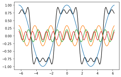
With more and more non-linear equipment getting added to the grid, for instance, converter-driven equipment, notably motor drives and consumer electronics, there is an increased occurrence of excessive harmonics getting introduced into the system. Why this happens is pretty easy to understand. Converter driven equipment often produce non-sinusoidal periodic signals, which are in principle, composed of an infinite number of sinusoidal signals (Fourier's theorem). These devices, using rectifiers and other converters produce multiples of the fundamental frequency (50 Hz, or 60 Hz, depending on the utility). Excessive harmonics in the system can lead to overheating of transformers, produce ‘electromagnetic noise’ that can interfere with sensitive electronic equipment, and reduce the output of several devices.

Smart Grids are emerging as an alternative to conventional grids. They would need to meet the increasing need for reliable, efficient and high-quality power. This though, is made difficult because of integration of renewable energy sources, storage units, controllable loads, with the grid, which add to the power quality disturbances present in the system. To meet the goals, one needs devices to mitigate the effects of power quality fluctuation. And for that, one needs to properly identify the types of power quality disturbances, and the sources thereof. This necessitates for the operators to continuously monitor and identify these disturbances. The popular methods include application of signal processing techniques to extract features from the voltage signal, which are later used to classify the disturbance by using soft computing techniques.

Since knowing one’s nemesis is the first step towards countering them, let’s move ahead and classify power quality disturbances into convenient categories.

Identifying the nemeses…

Power quality can be described as the grid’s ability to supply clean, reliable power, free from distortions. The voltage and current waveforms for all appliances should remain (nearly) sinusoidal. To characterise the ‘quality’ of power supplied, we look into the symmetry, frequency, amplitude of the waveforms.

The above definition provides a way to characterise power quality ‘disturbances’

1. Voltage amplitude variation: On an average, the voltage amplitude values are equal to their average specified values, but they are never equal. The variation in voltage during a day can be specified using a distribution function. The steeper the distribution is about the mean, the better is the quality of the voltage supplied. Voltage magnitude variations can be caused by a variation of load in a section of the grid.
2. Current amplitude variation: As stated earlier, current magnitude variations in a section of the grid can lead to voltage amplitude variations. As is evident from the name, the current amplitude values change throughout the day. The design of the power distribution system depends on the variation in the current amplitude within the system.
3. Voltage frequency variation: A difference in the generated power and load, causes frequency imbalances. Frequency transients introduced due to short circuits in a system are also included in this category. The frequency is never constant, but varies around the mean value.
4. Voltage and current imbalance: Three phase systems need the voltage supplied in the three phases, as well as the phase between them to be equal. Any deviation from the above criteria falls under this category. This is caused mainly due to load imbalances, which refer to an asymmetric distribution of load among the three phases. This is a serious concern for three phase loads. This leads to excessive heating of wires in induction and synchronous machines, thus reducing their efficiency.
5. Voltage fluctuation: Voltage fluctuation, or voltage flicker is defined as high frequency (which in the present context would mean any variation in the span of a few seconds) voltage variation. This leads to a reduction in device performance, but isn't directly noticeable, unless we are talking about tube lights/bulbs. For instance, if the frequency of the fluctuation is between 1 Hz to 10 Hz, it is directly noticeable by the human eye and can be quite irritating. The sensitivity of human eyes to high frequency fluctuations, explains the interest in this phenomenon, as well as its naming as ‘voltage flicker’.
6. Harmonic current and voltage distortions: Presence of non-linear loads in the system produces harmonics, which are multiples of the fundamental frequency. These are a serious concern, because they lead to excessive heating and thus losses in the appliances.
7. Interharmonics: Several appliances like arc furnaces, and physical phenomena like changes in Earth’s magnetic field following a solar flare, introduce frequency components that aren’t multiples of the fundamental frequency. They can damage the appliances operating on the grid, and thus present a serious concern while dealing with power quality disturbances.
8. Voltage notching: Use of appliances such as rectifiers can cause a drop in supply voltage during the commutation interval, that is the period when the current shifts from one thyristor in the rectifier to the next. In ideal circuits, the shift of current from one thyristor to the next is instantaneous. But, inductance in the supply, doesn't allow for an instantaneous change in the value of current flowing through a thyristor. This leads to voltage notching. This is a periodic phenomena, that leads to high frequency components in the voltage waveform.

Now several of these disturbances, for instance, voltage notching can either occur for short durations of time, while others like frequency variation, voltage fluctuation, interharmonics persist for longer intervals. Clearly, simple frequency domain analysis is insufficient for characterisation and classification of the disturbances, since the disturbances can span for varying periods.

Looking at time and frequency simultaneously…

We are all familiar with the ‘Fourier transform’. It provides us with an elegant way to decompose a signal into harmonics, and find relative strength of different harmonics in a signal. While it helps in analysing how the signal appears in the frequency domain, it fails to identify the temporal location of a disturbance ‘event’. Also, it isn’t useful for short bursts of signals, which don’t span over a large duration. Since the above two phenomena are one of the power quality disturbances that we encounter, a transform that enables us to look at time and frequency simultaneously is required.

An alternative to the Fourier Transform is the Short time Fourier transform. Here, we fix a window length, and take the Fourier transform of the signal in that window. Thereafter, we shift the window to different locations to obtain the spectra at different times. We would obtain a three-dimensional graph as a consequence, telling us about the temporal as well as spectral information contained in the signal.

The short time Fourier transform has one limitation in its window size. The width of the window wherein you find the Fourier transform of the signal is fixed. Thus, with narrow windows, you can’t capture low frequencies (since a waveform with low frequency would take a longer time span to complete one period), and thus, low frequency differences. The frequency resolution with narrow windows is low. At the same time, large windows would make it impossible for us to detect ‘events’ that don’t last for more than a few milliseconds, thus reducing the time resolution.

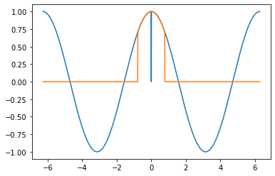
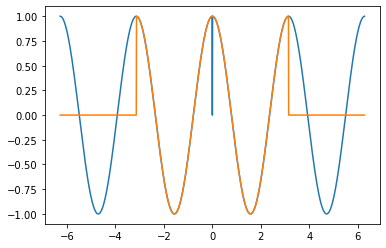
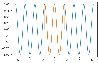
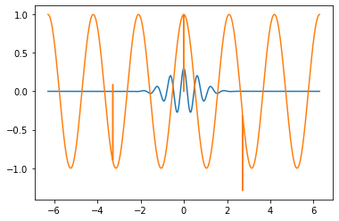
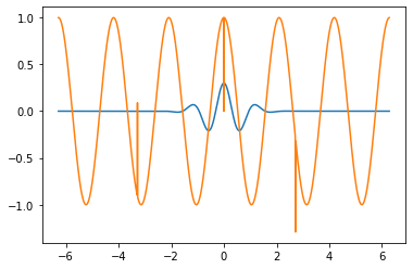
An alternative to the STFT is presented by wavelet transforms. Instead of using a window, we use wavelets with different scales. A wavelet is an oscillation that persists for a short period of time. It begins at zero amplitude, increases in amplitude to a certain limit, and then falls off’.

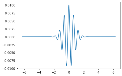
A wavelet can be scaled, as well as shifted in time. This thought forms the basis of wavelet transforms. A wavelet with a larger scale (one having a larger frequency of oscillations) would be able to capture a higher frequency resolution. A wavelet with a smaller scale, on the other hand would be able to capture a higher time resolution. Thus, the shortcomings of the STFT are done away with.

There are discrete versions of the wavelet transform that are implemented by passing the signal through low pass and high pass filters to separate out different frequency constituents. This is followed by down sampling (reducing the sample size of the signal) to half the previous value.

Wavelet transforms are ubiquitous in signal processing. They are used for high-fidelity signal compressions, signal denoising, and detection of discontinuities in the signal. A modified version of the discrete wavelet transform, called Tunable Q wavelet transform was suggested by Ivan W Selesnick. It can be used to extract different features from a voltage signal, which can later be used to classify the power quality disturbance in the signal. The Quality factor of the filters can be adjusted using this method, depending upon the oscillatory behaviour of the signal being fed in.

You know some, you learn some…

Given the problem of making a system to classify something into a given class, you have two different ways you could go about doing it.

1. Hardcode the rules in the form of domain knowledge, and feed them to the system. The system would use the rules to perform classification.
2. Collect a set of examples which have already been classified, and use that knowledge to ‘teach’ the system how to perform classification. In this case, the system learns the rules on its own.

Now both of these approaches have some upsides and downsides. For the former, there is an implicit assumption that the knowledge about the process is complete and correct. But for real world examples, achieving either or both among completeness and correctness is a difficult task. Even when the rules are specified to get a desired level of accuracy in performing the task at hand, they can become really complex and branched. Thousands of interrelated, or worse, recursive rules can result, keeping track of which could become a herculean task. Also, for any change in input data, we might need to modify the system, which for a system having several complex linkages might turn out to be an exercise in masochism.

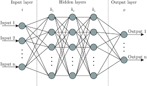
We can turn to empirical learning approaches to avoid the issues with the first approach. What do we observe then? We need huge amounts of data. The system can learn the rules on its own, but needs a lot of examples to attain a desired level of accuracy. Also, making the data more and more general is a difficult task, without which, certain biases might creep into the system. Artificial neural networks are one among the many paradigms under the empirical learning approach. They, in addition to the problems mentioned ahead, require long training periods and a problem-specific topology.

Hybrid learning systems, bring the best from both approaches together. They use the fact that the shortcomings in one approach is complemented by the latter. For instance, we can begin with simpler rules and then allow the empirical learning to take over and learn more complex rules, building over the ones given beforehand. At the same time, the training times are lowered since we don’t have to begin from scratch.

This is the motivation behind using Knowledge based Artificial neural networks (KBNN) for the task of classifying the power quality disturbance.

What have the other researchers done?

Diagnosis and characterisation of signals requires two steps. First, preliminary analysis and feature extraction from the signal that would be fed into the classifier model. Second, training the classifier model, and validation post the completion of training. For the former, methods like Fast Fourier transform (FFT), discrete wavelet transform (DWT), Wavelet packet transform (WPT), Empirical mode decomposition (EMD), Kalman filter and Stockwell transforms (ST) have been applied, and the results have been published. FFT, as we mentioned earlier, can’t give temporal information about the signal, which might be crucial for locating transient power quality disturbances. WPT and DWT are good options, but they suffer from the problem of pre-defined filter design (non-adjustable) and thus the extracted components cover a wide band of frequencies. They can’t distinguish between some disturbance categories if the signal has a low SNR. EMT and ST both suffer from the problem of mode-mixing, and thus aren’t great options either.

The Tunable Q- wavelet transform described in the previous section, can be used for extraction of the fundamental frequency component, since the filter design can be adjusted for extracting the fundamental frequency component, and other higher order harmonics from the distorted signal.

For the classification problem, several approaches have been suggested and tried. These include decision trees, rule based expert systems,  fuzzy logic, K nearest neighbours, support vector machines, and artificial neural networks. Decision trees and rule based expert systems assign equal weightage to all the features in classification. This can increase the possibility of an error in classification. An Artificial Neural Network is an attractive option, because of the flexibility offered in terms of weights assigned to different features. But as stated in a previous section, training and deciding the structure of the network is a laborious exercise, and requires a huge dataset.

A novel approach…

In their paper in 2018, Dr Trapti Jain, Dr Amod Umarikar, associate professors at IIT Indore, Karthik Thirumala, a research scholar at IIT Indore, and M Siva Kumar, an undergraduate student at IIT Indore, applied TQWT (Tunable Q Wavelet Transform) for preliminary analysis and feature extraction from the distorted signal. They used a dual multi-class SVM classifier for classifying the disturbance from one among 14 classes, as under:

C1 – voltage fluctuation, C2 –voltage fluctuation with harmonics, C3 – voltage fluctuation with transient, C4 – voltage interruption, C5 - sag, C6 - swell,C7 - harmonics, C8 - oscillatory transients, C9 - notch, C10 -spike, C11 - sag with harmonics, C12 - swell with harmonics, C13 - sag with transient and C14 - swell with transient

While previous approaches with SVM classifier had required more than 5 extracted features for classifying less than ten disturbance categories. By using a dual Multi class SVM (MSVM) classifier, they were able to obtain decent accuracies with just 5 features, and classify the disturbance into one of the above 14 classes. The MSVM classifier uses a lesser number of binary SVMs, thus leading to a faster classification. Also, the issues with other approaches, as explained before are averted. They obtained an average accuracy of 98.78% with noiseless signals and 96.42% with a noisy signal.

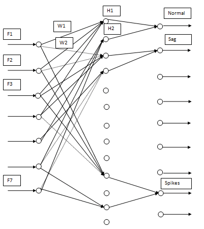
In a later paper, in 2019, Dr Amod Umarikar and Dr Trapti Jain, along with Karthik Thirumala and Harshal Jamode, from NIT Tiruchirappalli used a wavelet packet transform for extraction of the fundamental component from the distorted signal. Using seven features, they used a knowledge based neural network (KBNN), a hybrid learning system, for classifying the power quality disturbances into six classes. The KBNN used a rule based connectionist approach, which decided the no of layers of the neural network, and the no of nodes in the input and output layers. The rules were defined based on available literature. After that, they trained the neural network with a backpropagation algorithm to set the weights and biases for the hidden layers. Using the final neural network as a classifier, they were able to obtain 99.33% accuracy for the classification into six classes, as under:

C1- Normal voltage, C2- Voltage interruption, C3 - Voltage Sag, C4- Voltage Swell, C5 - Harmonics C6- Oscillatory transients.

Their next paper, in 2019, brought together the application of TQWT for preliminary analysis of the signal and feature extraction, and knowledge based neural network (KBNN) for the classification. Seven extracted features were used for classification of the distorted signal into nine categories. The procedure for building the preliminary connectionist network, and training the network on a dataset, were the same as explained in the previous paragraph. They were able to obtain a classification accuracy of 98.33% for classification into nine classes, as under:

C1- Normal voltage, C2- Voltage interruption, C3 - Voltage Sag, C4- Voltage Swell, C5 - Harmonics C6- Oscillatory transients, C7-Voltage fluctuation, C8-Notch and C9-Spike

Conclusion

A perfunctory glance might make the above seem like a purely academic exercise. But, the classification of the power quality disturbances serves a practical purpose. First of all, it helps in quantification of power quality. Next, for developing appropriate mitigating devices for reducing the effect of these distortions, one needs an understanding of their types and sources. There lies the importance of classifying the disturbance into various categories and finding ways to do the categorisation more accurately. After all, countering one’s nemesis requires one to know their modus operandi, and that’s what researchers working in this arena have been trying to do.